Grokking Recursion Through SQL

14 minute read

title_fib_q

Introduction

I have a controversial take for today. If you struggle with understanding fixed points, ~~you just need to understand them first~~ reverse engineering SQL’s recursive CTEs can be very beneficial.

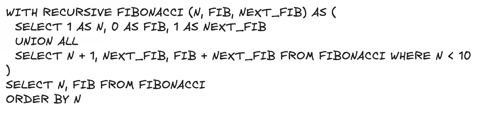
Recursive CTEs are queries that use themselves as part of implementation, for example:

WITH RECURSIVE FIBONACCI (N, FIB, NEXT_FIB) AS (   
  SELECT 1 AS N, 0 AS FIB, 1 AS NEXT_FIB  
  UNION ALL  
  SELECT N + 1, NEXT_FIB, FIB + NEXT_FIB FROM FIBONACCI WHERE N < 10
)  
SELECT N, FIB FROM FIBONACCI  
ORDER BY N

Recently I worked on implementing recursive queries for a custom SQL dialect. For the first few days, I was quite proud of myself: “Hey, I can tackle this because I have a good understanding of how recursion works.” But then I realized that the underlying components are actually simple to handle because SQL’s building blocks are ought to be precise and unambiguous. The reality was the opposite of what I expected — even if I had no prior knowledge of recursions and fixed points, I would have become familiar with them as a side effect of this work.

I discovered that approaching the “recursion problem” through SQL-related implementations is a non-obvious but straightforward way to build a mental model around it.

In this post, I’ll cover:

Quick Apache Calcite set-up (won’t be part of the post, but the linked repo has all the code) to parse recursive queries
Studying relational nodes that represent recursion in logical plans, examining what contracts they provide and how they decorate fixed points

Note 1. I am not going to make full cycle and compile a query back to some dialect. Main focus is to show how relational nodes represent recursion.

Note 2. If you like to work on problems like this (tweaking logical plans, crafting custom SQL dialects, etc.), you might be interested in globally remote Senior/Staff Backend Engineer - Query Compiler job opening at Narrative I/O. Feel free to reach me out in case of questions.

Parsing step

I’ll use Apache Calcite to parse and transform the query. You don’t need to know the configuration details, but all code is available in the project if you want to download and run it yourself. The link: https://github.com/antonkw/rec-cte-demo

val fibonacci =
"""
  |WITH RECURSIVE FIBONACCI (N, FIB, NEXT_FIB) AS (
  |  -- Base case: first two Fibonacci numbers
  |  SELECT
  |    1 AS N,
  |    0 AS FIB,
  |    1 AS NEXT_FIB
  |
  |  UNION ALL
  |
  |  -- Recursive case: generate next Fibonacci number
  |  SELECT
  |    N + 1,
  |    NEXT_FIB,
  |    FIB + NEXT_FIB
  |  FROM
  |    FIBONACCI
  |  WHERE
  |    N < 10  -- Generate first 10 Fibonacci numbers
  |)
  |
  |-- Select the sequence
  |SELECT
  |  N,
  |  FIB
  |FROM
  |  FIBONACCI
  |ORDER BY
  |  N
  |""".stripMargin

val fibonacciSqlNode: SqlNode = Calcite.parseQuery(fibonacci)
println(fibonacciSqlNode)

/*
WITH RECURSIVE `FIBONACCI` (`N`, `FIB`, `NEXT_FIB`) AS (SELECT 1 AS `N`, 0 AS `FIB`, 1 AS `NEXT_FIB`
UNION ALL
SELECT `N` + 1, `NEXT_FIB`, `FIB` + `NEXT_FIB`
FROM `FIBONACCI`
WHERE `N` < 10) SELECT `N`, `FIB`
FROM `FIBONACCI`
ORDER BY `N`
*/

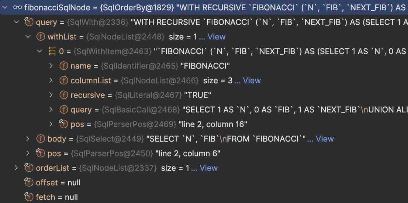
While we’re not particularly interested in syntax-level nodes today, I’ve included the screenshot to demonstrate how this query is represented by a SqlOrderBy node that contains other nodes like SqlWith, SqlNodeList, SqlWithItem, etc.

It’s worth noting that SqlWithItem has an explicit literal to mark recursive CTEs.

fib

And to accomplish the formal “syntax loop,” let’s validate the query and reformat it.

val validatedNode: SqlNode = Calcite.validate(fibonacciSqlNode)  
val formatted = Calcite.prettyPrint(validatedNode)

Output:

WITH RECURSIVE FIBONACCI (N, FIB, NEXT_FIB) AS (SELECT
        1 AS N,
        0 AS FIB,
        1 AS NEXT_FIB
      UNION ALL
      SELECT
        N + 1,
        NEXT_FIB,
        FIB + NEXT_FIB
      FROM
        FIBONACCI
      WHERE
        FIBONACCI.N < 10) (SELECT
      N,
      FIB
    FROM
      FIBONACCI
    ORDER BY
      N)

Relational nodes

Logical plan

Finally, we reach the point where we can build relational nodes and see how the logical plan looks like:

val relationalNode: RelNode = Calcite.convertSqlToRel(validatedNode)  
val logicalPlanPrinted = relationalNode.explain()  
println(logicalPlanPrinted)

LogicalSort(sort0=[$0], dir0=[ASC])
  LogicalProject(N=[$0], FIB=[$1])
    LogicalRepeatUnion(all=[true])
      LogicalTableSpool(readType=[LAZY], writeType=[LAZY], table=[[FIBONACCI]])
        LogicalValues(tuples=[[{ 1, 0, 1 }]])
      LogicalTableSpool(readType=[LAZY], writeType=[LAZY], table=[[FIBONACCI]])
        LogicalProject(EXPR$0=[+($0, 1)], NEXT_FIB=[$2], EXPR$2=[+($1, $2)])
          LogicalFilter(condition=[<($0, 10)])
            LogicalTableScan(table=[[FIBONACCI]])

If you’re not familiar with the concept of logical plans, this output might seem unreadable. I’ll try to explain it from the bottom up, focusing on the essential details.

LogicalTableSpool(readType=[LAZY], writeType=[LAZY], table=[[FIBONACCI]])
    LogicalValues(tuples=[[{ 1, 0, 1 }]])

LogicalValues represents inputs for the first round of recursion: SELECT 1 AS N, 0 AS FIB, 1 AS NEXT_FIB. It is our “seed” that will be use as starting value-set.

Table Spool

The LogicalTableSpool is one of the “helpers” that shows recursion from a different angle. Let’s look at the documentation.

From org.apache.calcite.rel.core.Spool:

/**  
 * Relational expression that iterates over its input and, in addition to * returning its results, will forward them into other consumers.*/ 
public abstract class Spool

From org.apache.calcite.rel.core.TableSpool:

/**  
 * Spool that writes into a table.*/
public abstract class TableSpool

Spool also defines write and read types:

/**  
 * How the spool consumes elements from its input. 
 * - EAGER: the spool consumes the elements from its input at once at the initial request 
 * - LAZY: the spool consumes the elements from its input one by one by request.  
 */  
public final Type readType;  
  
/**  
 * How the spool forwards elements to consumers.
 * - EAGER: the spool forwards each element as soon as it returns it;  
 * - LAZY: the spool forwards all elements at once when it is done returning all of them. 
 */  
public final Type writeType;

The abstraction of a “spool” is somewhat novel because a typical recursive function doesn’t expose any notion of cache needed to store intermediate results. You can manually introduce tail recursion and an accumulating structure, but generally, we rely on stack frames to handle our intermediate values (until a StackOverflow occurs :) ).

Coming back to TableSpool, we can think of it as a cache for recursive query results. It helps with incremental evaluation and stores intermediate rows between iterations.

Repeat Union

At this point, it’s time to examine LogicalRepeatUnion because these components work together.

/**  
 * Relational expression that computes a repeat union (recursive union in SQL terminology).
 * This operation is executed as follows: 
 * - Evaluate the left input (i.e., seed relational expression) once.  
 * - Evaluate the right input (i.e., iterative relational expression) over and  
 *   over until it produces no more results
 */
public abstract class RepeatUnion extends BiRel

It operates by repeatedly unioning the base case rows with the recursive case rows until a fixed point is reached.

LogicalRepeatUnion describes the union of:

Newly generated rows from the recursive case
The accumulated result set

Union meets Spool

This union continues until no new rows satisfy the termination condition—formally reaching a fixed point. I want to emphasize that each individual step processes newly generated row(s) while all previous results are accumulated in a transient table.

To round up, let’s recall how those new rows are being projected from the transient table:

LogicalProject(EXPR$0=[+($0, 1)], NEXT_FIB=[$2], EXPR$2=[+($1, $2)])
  LogicalFilter(condition=[<($0, 10)])

Here we have:

A filter which is effectively responsible for stopping the processing (no new rows are returned after N reaches 10)
Expressions being applied to the retrieved results to generate the next Fibonacci numbers

And this is still just a logical plan. We’re not discussing actual execution yet. However, the plan describes the nature of the processing and should be unambiguous for further interpretations.

Optional iteration limit

Since this is a generic pattern rather than a particular physical implementation, some flexibility remains. For example, let’s examine the constructor of the node itself in the codebase:

LogicalRepeatUnion create(
	RelNode seed, 
	RelNode iterative,  
    boolean all, 
    int iterationLimit, 
    @Nullable RelOptTable transientTable
)

The process typically terminates when no new rows satisfy the condition, not by hitting a maximum iteration count. Nevertheless, iterationLimit exists and the node can specify an allowable number of iterations. In our case, the limit is automatically set to -1, as we derived the plan from a query that doesn’t specify it.

Recursive CTEs aren’t standardized across all SQL implementations, so iteration limits often can’t be specified directly in the query. However, some dialects do support this functionality. For example, Transact-SQL provides the MAXRECURSION query-level hint.

Conclusion

By examining the nodes like LogicalTableSpool and LogicalRepeatUnion, we can see how SQL implements recursion through explicit caching and union operations. I personally liked working with Calcite’s abstractions built to represent recursions. While they are quite verbose and restricted by SQL’s abstractions, those dependencies and verbosity gives a different (very simple in my opinion) angle at recursion. I hope you found it useful and/or fun as well.

Anton Kovalevsky